GFlowNets and Scientific Discovery
A high level overview of GFlowNets and their potential to accelerate scientific discovery.
(This a high-level summary of our recent paper
The Scientific Method
“Science is often described as an iterative and cumulative process, a puzzle solved piece by piece, with each piece contributing a few hazy pixels of a much larger picture.” — Emperor of all Maladies, Siddhartha Mukherjee
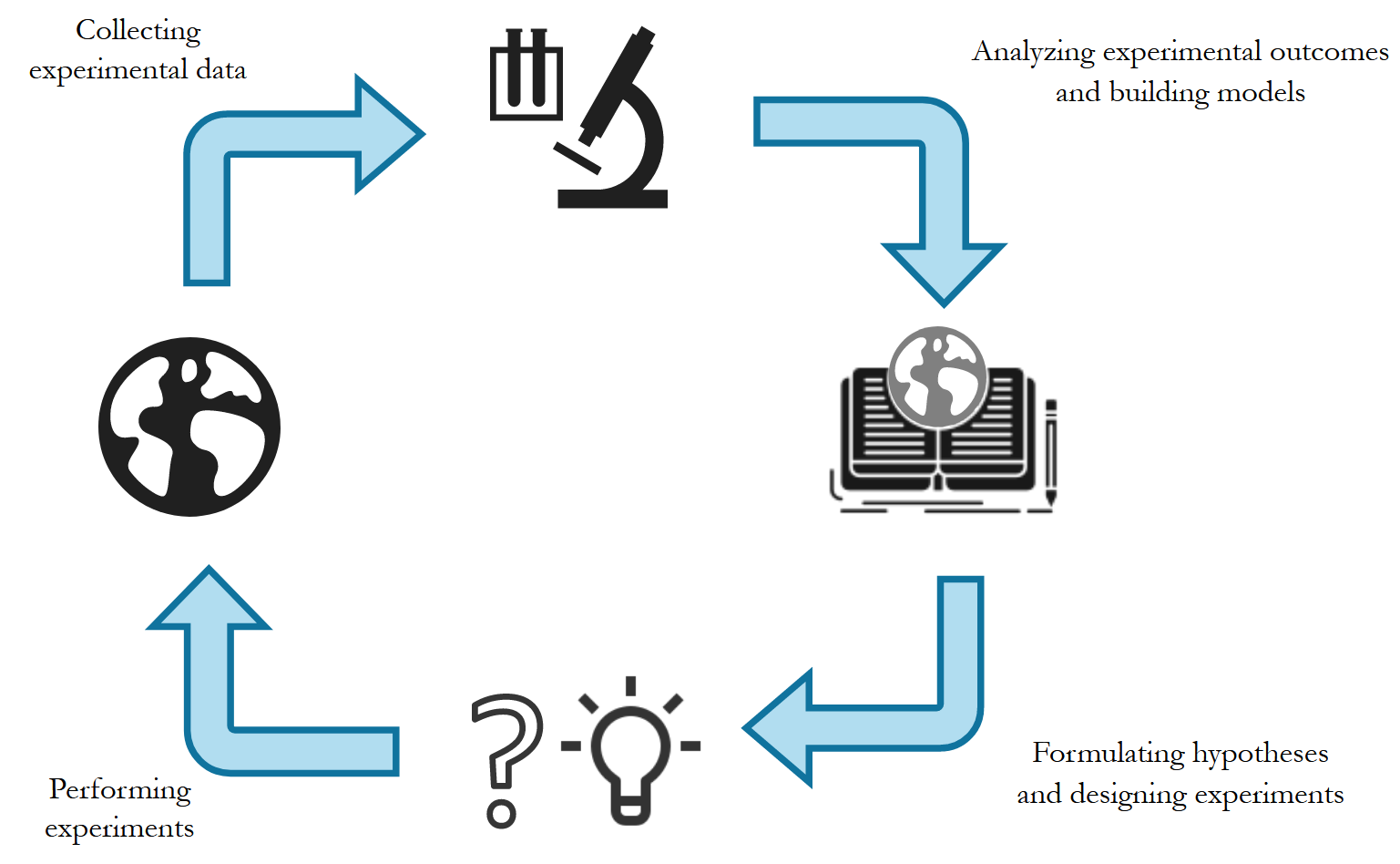
The Scientific Method prescribes a systematic approach to gaining knowledge through observation, forming hypotheses, and experimentation. Popularized during the Renaissance, this principle has been at the core of the rapid technological growth that followed. Progress in science has led to technological advancement, which in turn has enabled further scientific progress, resulting in a continually improving “hazy picture” of the universe. Figure 1 shows a simplified version of the Scientific Method.
To make the illustration concrete, consider the drug discovery process. It begins with the observation of a phenomenon in nature - the symptoms of a disease. These observations are then incorporated into our existing models of biology and medicine. Based on these observations and prior knowledge, several hypotheses can be formulated regarding the disease - the cause, mechanism of action, and potential therapies. These hypotheses are tested through experiments - detecting the presence of viral agents in affected organs, observing genetic pathways, testing therapies on isolated cells in-vitro, etc. At this point, completing the cycle, we return to the phase of observation, this time considering the effect of the designed experiment on the phenomenon. This cycle results in a constantly improving understanding of the phenomenon - improving our knowledge about biology and medicine, and increasingly precise and effective experiments - leading to better therapies.

Experimentation and Computation
The scientific method can be viewed as two complementary phases of computation and experimentation. Experimentation serves as an interface to the real world, where the phenomenon of interest is observed, intervened upon and its effects measured. Computation consists of analyzing the observations and experimental outcomes, formulating hypotheses and designing experiments to test said hypotheses. In reality the distinction between the two is often blurred. Computation and experiment have a symbiotic relationship - each one is incomplete in isolation without the other - which ultimately leads to progress. Historically, each of these phases can take considerable amounts of time. However, advancements in natural sciences have revolutionized the scale and precision with which experiments can be performed. At the same time advances in fields like machine learning have opened new avenues to accelerate computation. In this post, we focus on methods that enable us to accelerate the computation phase with data-driven approaches.
Predictive Modelling and Reasoning
The computation phase deals with two distinct problems:
- Building models of the environment in which the phenomenon occurs: This approximate model should be expressive, capturing all aspects of the environment influencing the phenomenon. As the model will be built with finite experimental data, it should also be able to capture it’s epistemic uncertainty.
- Reason about the phenomenon of interest and formulate hypotheses and design experiments: Leveraging the approximate model, we would like to come up with hypotheses and experiments about the phenomenon of interest.
Recall the drug discovery example. Say we have identified a target protein responsible for the ailment, one can collect experimental data about the structure and binding behavior of the protein with ligands through in-vitro experiments, and build a computational model that captures this behavior, i.e. docking. Using this model, we can design ligands that can inhibit the activity of the said protein.
In reality, however, each of the steps in the example above are extremely non-trivial, resulting in long timelines for drug discovery. Recent developments in machine learning are an exciting avenue, as they enable us to build large-scale complex models of physical systems, formulate hypotheses and design experiments to accelerate the computational phase of scientific discovery.
Challenges
In the last few decades, machine learning has enabled remarkable technological advances ranging from superhuman Go players to protein folding. These advances have been enabled, in part, by availability of extremely large datasets. A lot of the the approaches also assume the availability of a well specified objective to optimize. This leads us to two critical challenges in leveraging ML approaches for scientific discovery.
Data
The first critical challenge in leveraging learning based approaches for scientific discovery is that of limited data. By design, machine learning approaches rely on access to large datasets to extract useful patterns. But owing to fundamental limitations, it can be extremely expensive or impossible to obtain large amounts of data in many applications of interest. Going back to the drug discovery example, it can be extremely difficult to obtain experimental data for small-molecules binding with a target protein, at the scale required for machine learning methods. Limited data introduces uncertainty in the models we can learn, which needs to be accounted for when formulating hypotheses with the model, as it can useful for guiding the search for novel hypotheses and experiments to disambiguate them. Bayesian models offer a principled approach to deal with limited data by modelling the posterior over functions that fit the data, however, owing to approximations required to scale to realistic data, they can underestimate the true uncertainty.
Underspecification and Diversity
Machine learning approaches often assume access to some reward signal to evaluate quality of designs. For instance, for designing drug-like molecules, the true objective is to find drug-like molecules that inhibit the target protein within the human body. This objective, however, potentially cannot be specified as a simple scalar reward. In practice, the binding energy of the molecule with the target protein is used as the reward signal to search for molecules. The binding energy alone cannot not account for a lot of the factors that can influence the effect of the drug molecule within the human body. Thus, a molecule that just minimizes this binding energy can provide no effect in the actual environment. This makes it critical to find diverse hypotheses (in this case molecules) to account for the underspecification and uncertainty in the reward signal. Widely used approaches to tackle such problems like reinforcement learning and Bayesian optimization aim to discover a single maximizer of the the reward signal, not accounting for underspecification of the reward signal itself.
GFlowNets
Generative Flow Networks (GFlowNets) are a recently proposed probabilistic framework to tackle these challenges. Originally inspired by reinforcement learning, GFlowNets model the sequential generation of compositional objects through a sequence of actions. GFlowNets aim to generate these objects proportional to a some given reward signal.
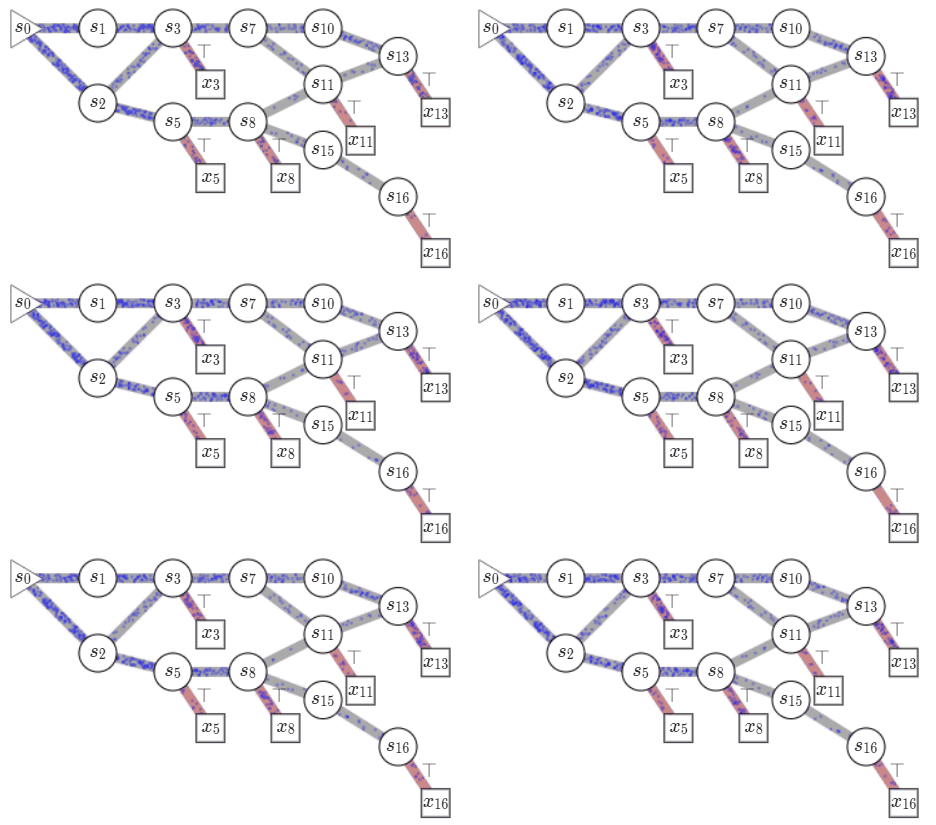
Consider a set of compositional objects \(\mathcal{X}\), for example, the set of all molecules \(50\) atoms. Each object \(x\in \mathcal{X}\) is composed of some building blocks \(\mathcal{A}\). In the molecule example, the building blocks consist of atoms and chemical bonds. Thus, each object \(x \in \mathcal{X}\) can be generated through a sequence of steps, where each step consists of adding a building block to an partially constructed object. In GFlowNets, we view this sequence of steps as a trajectory in \(\mathcal{G}\), a weighted directed acyclic graph (DAG), also known as a flow network in graph theory. The nodes of this graph, called states, consist of all possible objects that can be constructed using the blocks \(\mathcal{A}\), including an empty object \(s_0\) and partially-constructed. Any two states \(s, s'\) are connected by an edge \(s\rightarrow s'\) if there is a building block in \(\mathcal{A}\) that takes \(s\) to \(s'\). Note that building blocks available at each intermediate state can vary. In the molecule example, we cannot add a \(5^{th}\) bond to a carbon atom. Fully constructed objects \(\mathcal{X}\) are called terminal states i.e. have no outgoing edge, which in our molecule example corresponds to having the valency of all atoms satisfied. \(\mathcal{G}\) is acyclic since we are only allowed to add blocks, so we can never reach the same intermediate state again within a sequence.
Starting at the empty state \(s_0\), we can generate an object \(x \in \mathcal{X}\), by traversing \(\mathcal{G}\) till we reach a terminal state. We call this a complete trajectory, \(\tau = (s_0\rightarrow s_1 \rightarrow \dots \rightarrow x)\). There can be several trajectories, all resulting in the same object \(x\). Given a reward function \(R: \mathcal{X} \mapsto \mathbb{R}^+\), GFlowNets learn a stochastic policy \(\pi\) to generate trajectories such that an object \(x\) is generated with a probability proportional to \(R(x), \pi(x) \propto R(x)\). This policy is defined using flows on \(\mathcal{G}\) which are learned based on a principle akin to conservation laws in physics. A brief primer on learning in GFlowNets is provided in an Appendix at the end of the post but I recommend
This sampling of objects proportionally to the reward implicitly encourages generation of diverse and high reward objects, from different modes of the reward function. Within the context of the scientific discovery, GFlowNets can enable generation of diverse, good hypotheses and experiments, as well as building predictive models, discussed in the next section.

Why GFlowNets?
Let us look at how GFlowNets differ from other related conceptual frameworks:
- Reinforcement Learning: GFlowNets learn policies to sample trajectories to match the reward of the terminal state rather than maximize it as in standard deep reinforcement learning
- Markov Chain Monte-Carlo: GFlowNets amortize the computation during training so generating samples is fast, as opposed to MCMC methods where most of the computation happens during sampling. Additionally, GFlowNets exploit the generalization ability of neural networks potentially addressing the slow mode-mixing in MCMC methods.
- Generative Models: Traditional generative models in deep learning such as VAEs require positive samples to model the distribution of interest, whereas GFlowNets use a reward function.
GFlowNets roughly fall in the family of generalized variational inference methods and have strong connections to hierarchical variational models.
To summarize, GFlowNets shine in problems with the following properties:
- There is compositional structure that can be exploited by sequential generation
- There is uncertainty associated with the reward, and thus diversity is important
- The reward function of interest is multi-modal.
Learning in GFlowNets
Let us look at how we can learn \(\pi\). Each complete trajectory in \(\mathcal{G}\) is assigned a trajectory flow, \(F(\tau)\). This flow represents the unnormalized probability mass associated with the trajectory. We can also define the edge flow, \(F(s \rightarrow s') = \sum_{s\rightarrow s' \in \tau}F(\tau)\), which is the sum of flows of all trajectories containing the edge. A key idea in GFlowNets is using the flows to drive the sequential generation of objects. To this end, using the flows, we can define a forward policy \(P_F(-|s)\), which describes how to choose the next next action (addition of a building block) at a state. This forward policy is defined as \(P_F(s'|s)= \frac{F(s\rightarrow s')}{\sum_{s''\in\text{Child}(s)}F(s\rightarrow s'')}\).
We can generate trajectory \(\tau\) by iteratively sampling actions from the forward policy. As the actions at each state are assumed to be independent of the previous states, the likelihood of a trajectory under the forward policy is given by \(P_F(\tau) = \prod_{s\rightarrow s' \in \tau}P_F(s'|s)\). As noted earlier, there can be multiple trajectories resulting in the same object \(x\). The probability of generating an object \(x\) following \(P_F\), i.e. \(\pi(x)\) is given by \(\sum_{\tau=(s_0\rightarrow \dots\rightarrow x)}P_F(\tau)\), by considering all the trajectories resulting in \(x\). The learning problem in GFlowNets is to learn approximate flow functions such that the probability of generating \(x\), \(\pi(x)\) is proportional to its reward.
\[\pi(x) = \frac{R(x)}{Z}\]When this equation is satisfied, \(Z\) denotes the partition function of the unnormalized distribution represented by the reward function, \(Z = \sum_{x\in\mathcal{X}}R(x)\). Approaches to tackle this learning problem generally involve learning an approximate flow function, and or approximate forward policies. These are approximated with neural networks operating on states \(s \in \mathcal{S}\).
Flow Matching
A flow \(F\) is consistent if the outgoing flow at each non-terminal state \(s\) matches the incoming flow.
\[\sum_{s''\in \text{Parent}(s)}F(s''\rightarrow s) = \sum_{s'\in \text{Child}(s)}F(s\rightarrow s')\]This is similar to the notion of feasible flows in graph theory, and bears resemblance to the conservation laws in physics. Using this we can discuss a key result in GFlowNet, initially presented in
💡 Flow Matching Criterion
Given a consistent flow \(F\), with the incoming flow at terminal states set equal to the reward, \(\sum_{s'\rightarrow x\in \mathcal{E}}F(s'\rightarrow x) = R(x)\), the marginal likelihood of sampling an object \(x\) is proportional to the reward \(\pi(x) = \frac{R(x)}{Z}\).
In other words if the flow is conserved at all states, then sampling trajectories following the flow results in reward proportional sampling. This elegant result leads to a relatively straightforward approach for tackling the GFlowNet learning problem - learn parameters \(\theta\) for the edge flow function \(F(s\rightarrow s';\theta)\), which is typically a neural network - resulting in the following flow matching objective
\[\mathcal{L}_{FM}(\tau;\theta) = \sum_{s\ne s_0\in\tau}\left(\sum_{s''\in \text{Parent}(s)}F(s''\rightarrow s;\theta) - R(s) - \sum_{s'\in \text{Child}(s)}F(s\rightarrow s';\theta)\right)^2\]where \(R(s)\) is \(0\) for all terminal states and equal to the reward \(R(x)\) for the terminal states. We can already notice a key property of the learning objective - it is off-policy. What that means is that we can use any trajectory, not just ones sampled from the current policy, for training. This allows us to use exploratory policies to collect trajectories for training and even use offline data!
Subtrajectory Balance
Like temporal-difference learning objectives in RL, the flow matching objective, however, can suffer from slow credit assignment in long trajectories. This is addressed by the family of trajectory balance objectives. In particular, subtrajectory balance, introduced in
where \(\theta\) are the learnable parameters for \(P_F, P_B, F\). An interesting property of the objective is that it can operates on any subtrajectory. During training we consider subtrajectories from trajectroies sampled using the current policy. As opposed to the flow matching loss where credit is propagated over multiple trajectories, here the credit is assigned to all states in the subtrajectory resulting in lower variance in the gradients and faster convergence. I refer the curious readers to
We can define a general training algorithm for GFlowNets as follows
- Initialize parameters \(\theta\) for the flow function \(F(;\theta)\) and/or policies \(P_F(-|-; \theta), P_B(-|-;\theta), Z_\theta\)
- Sample trajectories following the forward policy \(\tau\sim P_F\)
- Compute loss for the trajectory \(\mathcal{L}(\tau;\theta)\)
- Update parameters \(\theta\) with gradients from the loss.
There is a growing literature around the mathematical foundations of GFlowNets which is too extensive to cover in a single post. I recommend
Promise of GFlowNets for Scientific Discovery
Generating Diverse and Useful Experiments
Our initial work on GFlowNets
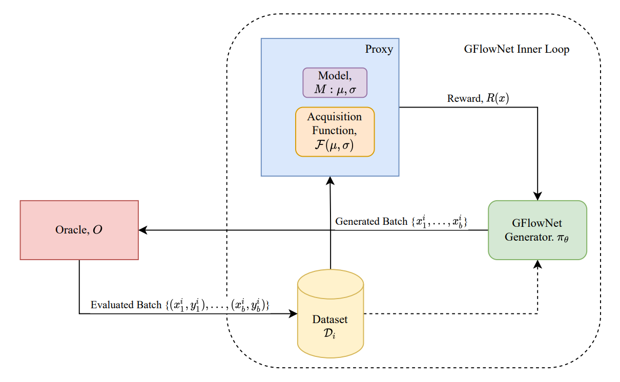
We looked at fragment based generation of molecules - the policy picks molecular subgraphs, rather than individual atoms, to put together for constructing the molecule graph. These fragments are generated from the Zinc database. This problem possesses all the 3 properties for GFlowNets to be effective - compositionality - the molecules are composed of the subgraphs with unique chemical properties, uncertainty in the reward - the reward is approximated by a neural network which will have some uncertainty associated to it, and the reward is multimodal - we can expect several molecules to bind well to a given target. Consequently, GFlowNets are able to substantially outperform other methods, generating diverse molecules with low binding energy. In particular GFlowNets discover significantly more modes of the reward function relative to other methods. Further we also consider an active learning setup where we start with a dataset of 2000 molecules and use the docking simulation as the oracle. We find that generating batches to be queried with GFlowNets results in significant performance improvements, resulting in discovery of much lower energy molecules than those in the initial dataset.
Further exploring the active learning setting, we considered additional improvements to GFlowNets to improve performance in the active learning setting

In many practical settings, there can be multiple properties of interest, where we want to generate experiments which capture them simultaneously. For example, in the context of drug discovery we would like to generate molecules that inhibit the target but which are also synthesizable and not toxic to humans. Multi-Objective GFlowNets
Learning Predictive Models
While still in early stages, recent work has also demonstrated the ability of GFlowNets to model predictive posteriors from data.
DAG-GFlowNets
Another popular paradigm for practical scenarios is that of approximate Bayesian inference. Methods such as Monte-Carlo dropout and ensembles have become default choices to represent the uncertainty over neural network parameters. Pushing this direction further, our recent work
Looking Forward
With this glowing discussion and diverse range of applications, you might be tempted to ask “Are GFlowNets all you need?” But as with most questions of this form, the answer is certainly “No”.
What GFlowNets do offer is a flexible probabilistic modeling framework that paves the way for developing approaches to accelerate scientific discovery. There are still several open challenges that need to be addressed in the context of GFlowNets: Multi-fidelity GFlowNets, Intervention Policies, Exploration, and many more! We expand on these ideas, positioning GFlowNets as a key tool to accelerate scientific discovery in
To get started with GFlowNets, checkout this tutorial Colab by Emmanuel Bengio, and this list of Awesome-GFlowNets by Dinghuai Zhang!
Acknowledgements
Yoshua Bengio and Emmanuel Bengio provided valuable comments and feedback on this post. My collaborators and mentors helped shape the ideas discussed here through numerous discussions.